Introduction to Tensorial 4.0  (version 2006)

Copyright 2006 Renan Cabrera, David Park, Jean-François Gouyet

Renan Cabrera
cabrer7@uwindsor.ca
Physics Department
University of Windsor
Ontario Canada

David Park
1429 Searchlight Way
Mount Airy, Maryland 21771, USA
djmp@earthlink.net

Jean-François Gouyet
Labo. PMC, Ecole Polytechnique
F-91128 Palaiseau Cedex, France
jean-francois.gouyet@orange.fr

Tensorial is a general purpose tensor calculus package for Mathematica Version 4.1 or later. We have tried to design it as an open system and natural extension of Mathematica, with routines that give access to all levels of tensor calculations. Thus it should be useful for students first learning tensor calculus and for advanced calculations. We also hope that the open design will make it easy to extend Tensorial to special purpose areas by adding subsidiary packages.

We consider Tensorial as a continuing project. Anyone who wishes to participate in the project should feel free to contact one of the authors above. We also appreciate any criticisms and suggestions.

The best starting point for learning Tensorial is the Tensorial Basics notebook in the Using Tensorial Help section.

Copyright & License Agreement

Tensorial and subpackages produced by the developers listed above are copyrighted by the developers.

Tensorial is licensed for single user use. Transfer of the Tensorial Mathematica package or subpackages to other persons is forbidden.

Tensorial and associated subpackages are provided on the condition that it is acknowledged that we accept no liability for software performance, continued maintenance, or damage to data. The authors retain any and all rights to the the Tensorial software and associated subpackages produced by the developers.

We request that if you make a publication extensively using Tensorial you reference the package and principal authors.

Design Principles

We have designed Tensorial on the following principles.

=>Tensorial must meld naturally with Mathematica and use the standard notebook interface. Users should be able to produce documents that follow normal textbook or research paper style.

=> No special symbols. No restrictions. For example, the base indices for a coordinate system can be any set of integers or symbols: {1,2,3} for 3D Cartesian coordinates, {0,1,2,3} or {t,x,y,z} for relativity problems, or {𝜌,𝜃,𝜙}for spherical coordinates.

=> No special tensor labels. You can use any labels you want for any kind of tensor. You can use δ for a Kronecker or you can use κ. You can use g for the metric tensor or you can use η. You can even have several types of Kroneckers or metric tensors in play at once. All the special properties of tensors are contained in the routines that process the tensors and not in their labels. This means that the intended labels must be fed to the routines. So MetricSimplify[g] will do metric simplification assuming that 2nd order tensors with the label g are metric tensors. MetricSimplify[ĝ] would use ĝ label tensors as metric tensors and not g label tensors. The disadvantage of this is that one has to feed the tensor labels to routines. The benefit is that you can be certain that no special definitions will be applied to a tensor just because you haplessly picked some label for it. You can adapt your notation to the field or textbook you are working in.

=> Coordinate systems are designated on the indices and not on the tensor labels. To facilitate this, index flavors have been introduced. An index flavor is either a color or an annotated symbol such as OverHat[i]. Thus you could have regular black indices for one coordinate system and red colored indices for another coordinate system. Sometimes it is nice to use colored indices just to make them better stand out. Flavored indices could also be used for other purposes. See the Index Flavors section in the Tensorial 4.0 Help to see how this is implemented. In Tensorial 4.0, each index flavor may also be associated with its own set of base indices and dimension.

=> One slot, one index. Every tensor, or indexed object, can have upper and lower indices. An upper index will always have a blank space below it, and conversely a lower index will always have a blank space above it. Although there is theoretical justification for just treating up indices and down indices separately and putting one above the other, the one slot - one index rule vastly simplifies the programming and reduces confusion. When a single upper index is lowered, without the rule, is it put at the beginning or end of the lower indices?

=> Normal Mathematica input is used with tensor shortcuts for tensors. The shortcuts are the minimum keystroke entry method for general tensors. The output is formatted, with a number of formatting options, and can be copied and pasted.

=> Some programming required. We are trying to build from the ground up by providing a convenient, versatile and rich suite of routines for manipulating tensor expressions and calculating the various derivatives. We have not yet provided automatic routines for every interesting tensor. We hope we have provided the tools so you can calculate the tensors that interest you.

=> Give Help. Documentation is as important as the code. We have provided regular Mathematica style documentation, with a Help page for each command as well as additional tutorial and example notebooks. Each help page contains examples for the command that illustrates its basic usage and we have occasionally attempted to slip in more advanced calculations. Using Tensorial\Tensorial Basics and then working through the Help pages will be the best way to learn Tensorial. The Flat and Curved example goes from very basic calculations to the calculation of curvatures and shows how text, derivation, calculation, graphics and animation can all be combined in a Mathematica notebook.

A Sample Calculation

Here we show a short calculation performed with Tensorial. In any notebook you will have to:
1) Load the package
2) Declare the base indices if they are different from the default.
3) Define tensor shortcuts for the tensors you will be using.
4) Declare any index flavors you will be using.

We will calculate the length of a specific curve on the surface of a sphere of radius a, described in spherical coordinates.

The Tensorial package can be loaded with the statement...

In[1]:=

We will use {𝜌,𝜃,𝜙} as our base indices.

In[2]:=

We define tensor shortcuts for the tensors we will use. x is a coordinate vector, v the velocity vector and g the metric tensor.

In[3]:=

We declare a red index flavor. red is the name of the flavor and Red is the actual RGBColor. (Graphics`Colors` is automatically loaded by Tensorial.)

In[4]:=

We define the metric tensor in conventional coordinates and then convert it to tensor coordinates.

In[5]:=

Out[5]//MatrixForm=

Out[6]//MatrixForm=

We then set rules for the values of the metric tensor. This is our first use of a tensor shortcut. gdd[red@a,red@b] specifies a tensor with label g and two down indices, "dd", which are a and b with the red flavor.

In[7]:=

We can look at the nonzero values with

In[8]:=

Out[8]//TableForm=

We also set value rules for the curve followed by x. Again we have used a tensor shortcut. xu[red@i] stands for the x tensor with an up index in the red flavor. The curve is at a constant radius a, and for 0≤t≤π moves from the North pole to the South pole while wrapping once around the sphere. We tell Mathematica and Tensorial that a is a constant.

In[9]:=

The velocity is the total derivative of the spherical coordinates.

In[11]:=

Out[11]=

Out[12]=

We set the velocity tangent vector to the total derivative of the coordinate vector.

In[13]:=

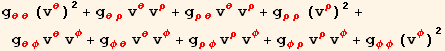
We now calculate the line element along the curve, using the tangent velocity vectors and the metric tensor. We do an Einstein summation and then substitute the tensor value rules for g, v and x. (This is a little tricky because we had to do multiple substitutions. x appears only after v is substituted.)

In[14]:=

Out[14]=

Out[15]=

Out[16]=

Out[17]=

The calculation could be shortened using the ToArrayValues routine.

In[19]:=

Out[19]=

Out[20]=

Out[21]=

Now we can calculate the length of the curve.

In[23]:=

Out[23]//StandardForm=

Out[24]=

Restore settings.

In[25]:=

Update History & Usage Changes

You may have both Tensorial 3.0 and Tensroial 4.0 installed. However, if the Help index is rebuilt with both packages and you select a command that is in both packages and use F1 to bring up the Help Browser, the browser will always direct you to 3.0 instead of 4.0. It is best to move Tensorial 3.0 out of the way, say to an InertApplications folder, and then rebuild the Help Index.

This section itemizes significant additions or changes in usage to Tensorial. See the relevant Help pages for full details of the commands.

New in Tensorial 4.0  - March 2006

All the output can now be copied and pasted. See UsingTensorial, Output Format.

Flavored indices can now be associated with their own base index sets and dimensions.

The output notation has been improved. Unexpanded partial derivatives now show only a single comma before the first differentiation index. Similarly an unexpanded covariant derivative shows only a single semicolon. (Other differentiation symbols can be used as before.) In addition there is an alternative mode of display for covariant derivatives using the ∇ symbol with subscripts. This can be turned on and off with SetCovariantDisplay. Similarly, SetLieDisplay can be used to display unexpanded Lie derivatives as a £ symbol with subscripts.

New commands have been provided in the Arrays section to facilitate the representation of tensor terms as products of actual vectors, matrices and arrays. This is called dot mode calculation.

The old Dif and Cov wrappers for differentiation indices are out. Unexpanded (to coordinates) partial and covariant derivatives are only broken out by their linear and Liebnizian properties and then left without further evaluation. This means that the old NestedTensor is unnecesssary and it has been removed. To prevent linear and Liebnizian breakout wrap the expression in Tensor instead of NestedTensor. UnnestTensor will still unwrap the expression.

An alternative, and perhaps better method to prevent automatic evaluation of built-in definitions is to use the new HoldOp command in the Functions & Rules section of Help.

DummySimplify has been removed. There is a new TensorSimplify. It selects terms that have the same pattern, applies any declared symmetries and then applies SimplifyTensorSum on these subsets of terms. UpDownAdjust can also be used to give a common up/down index pattern to terms with the same structure.

The Curvature section contains new routines (moved from the General Relativity subpackage) that calculate the Riemann tensor, up and down, the Ricci tensor, the scalar curvature and the Einstein tensor.

The new OrthonormalTransformation routine will, given a metric and a signature pattern, calculate a transformation matrix from the coordinated basis to an orthonormal basis.

A number of routines that are more in the class of general expression manipulation rather than tensor routines are gathered together in the Functions & Rules section. Two new routines here are SymbolsToPatterns and LHSSymbolsToPatterns. These are useful in turning derived equations into general rules that can be applied to subsequent expressions.

The $PrePrint for larger font output has been eliminated. Instead the Tensorial style sheet was changed to give a larger Output cell font. This simplifies copying and pasting by eliminating additional box structures. The style sheet was also changed to eliminate the Helvetica font in Headings in favor of Times. Some systems have a difficult time using the Helvetica font.

Also, in the Tensorial style sheet, Output cells are now StandardForm. Derivatives are formated in Leibnizian style but you will now have to use MatrixForm to format arrays.

The routines SetMetricValues, SetMetricValueRules, SetChristoffelValues and SetChristoffelValueRules have been removed. A new routine, CalculateChristoffels, calculates the Christoffel arrays and then SetTensorValues or SetTensorValueRules can be used to set the values. This provides a more uniform user interface that separates the calculation of values and the setting of values.

October 2006

HoldOp extended so the 'operation' can be a pattern. Peripheral fixes in ArrayExpansion, ExpandCovariantD and SymmetrizeSlots.

Usage of IndexChange changed slightly. NewIndexChangePatterns added to allow indices to be found in user defined structures.

A notebook on Customizing Tensorial was added to the Using Tensorial tutorials.

November - December 2006

PartialD and CovariantD usage changed so the the order of the differentiations cooresponds to the order of the indices taken left to right. This seems to conform to textbook usage even though it is opposite of the composition order. The differentiation indices in PartialD are no longer sorted.

An error in MetricSimplify that can occur when the tensor being simplified itself contains dummy indices is fixed.

A new routine SetScalarSingleCovariantD has been added that enables or disables the conversion of single covariant derivatives of scalar tensors to partial derivatives.

Created by Mathematica  (November 22, 2007)